Calculate Opponent Adjusted Strength

Audience: Basic knowledge about football and statistical modeling.

Introduction

---

I am going to employ many of the same techniques found in this blog post from collegefootballdata.com.

---

Evaluating a team's offensive and defensive capabilities is pivotal for assessing a team's success on the field. Expected Points Added (EPA), a metric calculated from Expected Points that we saw in my previous experiment, stands as a powerful metric for quantifying the impact of each play on a team's potential to score or prevent points. This experiment seeks to leverage EPA, employing a Ridge Regression model, to comprehensively measure the offensive and defensive strengths of NCAA football teams.

How is EPA different from Expected Points?
EPA is simply how much EP increases or decreases on each play, i.e. EP from the current play minus EP from the previous play. A positive EPA would indicate a succesful play as the team has increased their position in terms of scoring the next points.

Ridge Regression, a proven technique in predictive modeling, adds a valuable layer of sophistication to our analysis. By addressing issues of multicollinearity and overfitting, it ensures a robust and stable evaluation of team performance including the strength of their opponents.

By scrutinizing play-by-play data and applying Ridge Regression with each team as a predictor for EPA, we aim to offer a generalized assessment of a team's offensive and defensive strength. This methodology allows us to unearth nuanced insights, revealing not only how effectively a team scores, but also how effectively they prevent their opponents from doing so.

Data

The data that we are using comes from collegefootballdata.com. We are also leveraging the expected points data previously calculated. Cleanup and transformations have already been performed on the dataset and it only includes standard non-special teams plays, think passing and rushing plays.

EPA

import pandas as pd

df_epa = pd.load_csv('https://github.com/wsovine/data/blob/main/ncaaf_epa_pbp.csv')
							

Modeling with Ridge Regression

Use the team on offense, the team on defense, and homefield advantage (hfa) as our predictor variables (X) and Standard Expected Points Added (SEPA) as our dependent variable (y).

X = df_epa[['offense', 'defense', 'hfa']]
X = pd.get_dummies(X)

y = df_epa.sepa
							

We'll try out a few different values for alpha in the below code to find the one that minimizes RMSE. Alpha determines the strength of penalty term and the penalty term is what keeps our coefficients at a reasonable scale.

alphas = np.arange(10, 500, 10)
reg = RidgeCV(alphas=alphas, fit_intercept=False)

reg.fit(X, y)

print(f'{reg.alpha_ = }')
print(f'{reg.intercept_ = }')
print(f'{reg.best_score_ = }')
							

The next block of code simply takes the coefficients calculated in the above model for each team's offense and defense, averages out EPA for each team's offense and defense, and put it all in tabular form

df_results = pd.DataFrame({
    'coef_name': X.columns.values,
    'ridge_reg_coef': reg.coef_
})

# Offense coefficients
df_off = df_results[df_results.coef_name.str.startswith('offense')].copy()
df_off['coef_name'] = df_off['coef_name'].str.replace('offense_', '')
df_off.rename(columns={'ridge_reg_coef': 'adj_off_epa'}, inplace=True)

# Defense coefficients
df_def = df_results[df_results.coef_name.str.startswith('defense')].copy()
df_def['coef_name'] = df_def['coef_name'].str.replace('defense_', '')
df_def.rename(columns={'ridge_reg_coef': 'adj_def_epa'}, inplace=True)

# Extract each unique team to a dataframe
df_team_stats = (
    df_epa
    .rename(columns={'home_team': 'team'})
    [['team']]
    .sort_values('team')
    .drop_duplicates()
    .set_index('team')
)

# Tidy stats up in tabluar form
df_team_stats = (
    df_team_stats
    .join(df_epa.groupby('offense').sepa.mean())
    .rename(columns={'sepa': 'avg_off_epa'})
    )

df_team_stats = (
    df_team_stats
    .join(df_off.set_index('coef_name'))
    )

df_team_stats = (
    df_team_stats
    .join(df_epa.groupby('defense').sepa.mean() * -1)
    .rename(columns={'sepa': 'avg_def_epa'})
    )

df_team_stats = (
    df_team_stats
    .join(df_def.set_index('coef_name') * -1)
    )
							

Review the Output

Homefield Advantage

Before we dive into each teams strengths, lets first look at the extra predictor variable we added to the model to determine homefield advantage.

df_results[df_results.coef_name == 'hfa']
							

At around 0.007 points per play we can start to understand how big of an impact homefield advantage has.

Let's say there are 150 plays in a game, 75 plays for each team, we would expect about 1 point for the home team to be attributed to homefield advantage on average.

$$1.05 = 0.007_{hfa} * 75_{offense} + 0.007_{hfa} * 75_{defense}$$

Offense

Now let's check out the offense, we will take a glance at the top 5. Seems to make sense with Georgia at the top considering they did win the national championship.

(
    df_team_stats[['avg_off_epa', 'adj_off_epa']]
    .sort_values('adj_off_epa', ascending=False)
    .head()
)							

Defense

Next we check out the top 5 defenses. Annnnd things start to look a little fishy. Did James Madison of the Sun Belt Conference have a defense better than the national champions and the entire SEC for that matter?

(
    df_team_stats[['avg_def_epa', 'adj_def_epa']]
    .sort_values('adj_def_epa', ascending=False)
    .head()
)							

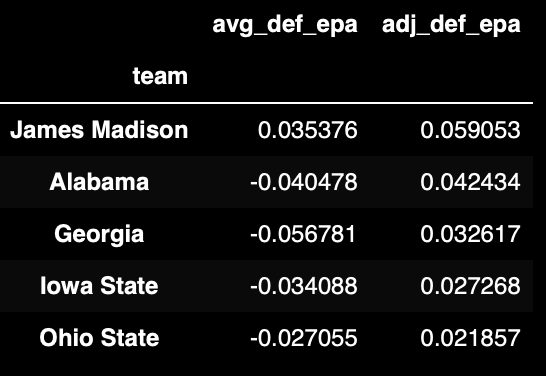
The outcome above reveals a big problem with this ridge regression method for calculating the opponent adjusted team strength. We have very sparse categorical data that we are trying to train this model with. Each game only allows us to compare two teams at a time, but that isn't even the biggest problem. Each team typically plays the majority of their games against opponents in their own conference and that doesn't allow us to adjust their strength relative to teams in other conferences very well.

In the above defensive strength output, there are 4 different conferences represented in the top 5 (Sunbelt, SEC, Big 12, Big 10). While it might make sense that JMU had the best defense in the SBC, you can't convince me that their defense would outperform Alabama's or Georgia's.

Adding Context

Let's add in the conference for each of our teams to at least give a bit of extra context around the team and their likely opponents.

teams_conf = pd.load_csv('https://github.com/wsovine/data/blob/main/ncaaf_fbs_team_conferences_2022.csv')

df_team_stats = df_team_stats.join(teams_conf)
							

Now we can plot our data using our 3 different dimensions (offense, defense, and conference) to really start to compare teams to one another.

import plotly.express as px

fig = px.scatter(
    df_team_stats.sort_values('Conference').reset_index(),
    x='adj_off_epa',
    y='adj_def_epa',
    color='Conference',
    hover_data=[
        'team', 'Conference', 'adj_off_epa', 'adj_def_epa'
        ]
    )

fig.add_hline(df_team_stats.adj_def_epa.median(), line_dash='dash')
fig.add_vline(df_team_stats.adj_off_epa.median(), line_dash='dash')

fig.update_xaxes(title='Offensive Effeciency', zeroline=False)
fig.update_yaxes(title='Defensive Effeciency', zeroline=False)


fig.add_annotation(
    x=df_team_stats.adj_off_epa.min(),
    y=df_team_stats.adj_def_epa.max(),
    text="Bad Offense | Good Defense",
    showarrow=False,
    yshift=20
    )

fig.add_annotation(
    x=df_team_stats.adj_off_epa.max(),
    y=df_team_stats.adj_def_epa.max(),
    text="Good Offense | Good Defense",
    showarrow=False,
    yshift=20
    )

fig.add_annotation(
    x=df_team_stats.adj_off_epa.max(),
    y=df_team_stats.adj_def_epa.min(),
    text="Good Offense | Bad Defense",
    showarrow=False,
    yshift=-20
    )

fig.add_annotation(
    x=df_team_stats.adj_off_epa.min(),
    y=df_team_stats.adj_def_epa.min(),
    text="Bad Offense | Bad Defense",
    showarrow=False,
    yshift=-20
    )
							

Try double-clicking the conference in the legend to filter down to that conference.

Conclusion

Ridge regression gives us a simple yet robust way to estimate opponent adjusted team strength for all teams at once. If falls short in certain areas with the sparsity seen in our dataset; however, we are able to overcome these challenges by adding in a bit more context to our interpretations.