Predicting Expected Points
Audience: Basic knowledge about football and machine learning models.
Introduction
What are expected points?
Expected points are how many points we can expect to be scored next, either by the current team on offense or the current team on defense (if expected points are negative).
Objective
Predicting expected points in NCAA football hinges on the nuanced situation of each play. Most models are based on the assumption that all yardlines are different and offer different expected outcomes, i.e. the closer you are to your opponents endzone, the more points you are likely to score. Machine learning (ML) models offer a potent tool to refine these forecasts. This experiment assesses various ML algorithms, prioritizing situational context integration. Our objectives are:
- Situational Context Integration:
Incorporate dynamic play factors (e.g., down, distance, field position) for precise predictions.
- Model Selection and Adaptation:
Evaluate models for adaptability to NCAA football's dynamic nature.
- Context-Specific Performance Metrics:
Employ tailored metrics for precise evaluation.
This research aims to enhance play-by-play analysis, empowering decision-makers with context-aware insights and enabling further advanced metrics for predicting outcomes.
Data
Load Data
The data that we are using comes from collegefootballdata.com. We are using the play-by-play data from the 2022 season and the first few weeks of the 2023 season. Cleanup and transformations have already been performed on the dataset, but it still isn't perfect and I think it is mostly due to the source which CFBD pulls the data from. However, I am hopeful that the noise of the imperfections will be muffled with such a large sample size.
import pandas as pd

df_pbp = pd.load_csv('https://github.com/wsovine/data/blob/main/expected_points_pbp.csv')
Process & Split Data
from sklearn.model_selection import train_test_split

X = df_pbp.drop('next_points_scored', axis=1)
y = df_pbp.next_points_scored

# one-hot encode the down variable, since it should be considered a categorical variable rather than a continuous variable
X = X.drop('down', axis=1).join(pd.get_dummies(X.down, prefix='down_'))

X_train, X_test, y_train, y_test = train_test_split(X, y, test_size=.3)
# EDA dataframe that we will use should only include our training data points so that we don not introduce any bias
df_eda = df_pbp.iloc[X_train.index]

print(f'{X_train.shape = }')
print(f'{X_test.shape = }')
print(f'{y_train.shape = }')
print(f'{y_test.shape = }')
EDA
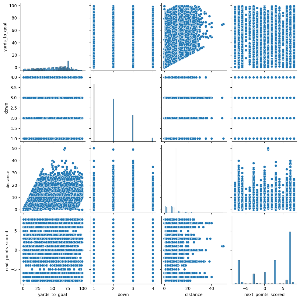
Yards to Goal
Yards to the other team's endzone.
Values seem to make sense. There is a high spike at 75 yards which would be
from teams starting at their own 25 yardline after a touchback.
The distribution seems to slope downwards towards either endzone
(i.e. 0 yards to goal and 100 yards to goal).
Down
What down the play is being run on.
We see first downs the most and fourth downs the least. This is intuitive
considering we expect a new first down every time a team starts their drive or
successfully gains ~10 yards. Fourth downs would be the least common since a team
needs to run 3 consecutive unsuccessful plays to reach a fourth down.
Distance
Yards needed for a first down or a touchdown.
Huge spike at 10 yards. Most every drive will start at 10 yards and then we see
10 yards again every first down. Distribution is bound at zero yards and we
see a right skew where distance is greater than 10 yards, these would result
from penalties or plays that went for a loss.
import seaborn as sns

sns.pairplot(df_eda)
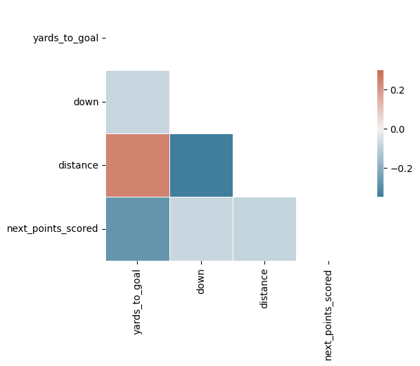
Correlation
Based on the above plots and explanations, I expect to see some correlation between our predictor variables. For example, a lot of plays that have 75 yards to goal are going to be first and 10 as this is the typical start of a drive after a kickoff or punt touchback.
import numpy as np

# Compute the correlation matrix
corr = df_eda.corr()

# Generate a mask for the upper triangle
mask = np.triu(np.ones_like(corr, dtype=bool))

# Generate a custom diverging colormap
cmap = sns.diverging_palette(230, 20, as_cmap=True)

# Draw the heatmap with the mask and correct aspect ratio
sns.heatmap(corr, mask=mask, cmap=cmap, vmax=.3, center=0,
            square=True, linewidths=.5, cbar_kws={"shrink": .5})
Linear Regression
This will be our baseline model. Simple linear regression using yards-to-goal as our predictor.
from sklearn.linear_model import LinearRegression

lr = LinearRegression()
lr.fit(X_train[['yards_to_goal']], y_train)

print(f"R2 = {lr.score(X_train[['yards_to_goal']], y_train)}")

y_pred = lr.predict(X_test[['yards_to_goal']])

rmse = mean_squared_error(y_test, y_pred, squared=False)
print(f'{rmse = }')

mae = median_absolute_error(y_test, y_pred)
print(f'{mae = }')
R2 = 0.078
RMSE = 5.232
MAE = 4.311
print(f'Intercept: {lr.intercept_}')
print(f'Coefficient: {lr.coef_[0]}')
Intercept: 5.185
Coefficient: -0.062
Predictability
The linear regression model using only the yards-to-goal predictor explains about 8% of the variance of the next points scored and the predictions are off by 4.3 or 5.2 points, depending on which error metric we look at, on average.
Explainability
A linear regression model does have the benefit of being very explainable. It tells us that on average, as the offensive team advances 1 yard closer to the opponents endzone, the next points scored increases by 0.06. With this model, we can say that every yardline is worth 0.06 points and we could start to measure a team's efficiency on each play.
For example: Your team starts with the ball on their own 25 yardline. On their first play, they run the ball for a 5 yard gain. Using our above model, they have increased their expected points by 0.3. $${ExpectedPointsAdded} = {yards\_gained} * 0.06$$ Do that 10 more times, and you've got yourself a field goal (0.3 * 10 = 3 Points). This seems to make sense as they would be on the opponents 25 yardline, certainly in field goal range. In fact, they would be a little above those expected 3 points at the opponent's 25 yardline when we factor in the intercept of 5.2. At the opponent's 25 yardline, the expected points are 3.7. $${ExpectedPoints} = {yards\_to\_goal} * -0.06 + 5.2$$
LASSO Regression
Next, let's see if adding more independent variables to our model helps with prediction.
Why not add more predictors to the linear regression model?
My concern with that is multicollinearity. There is some level of correlation between our independent variables and LASSO works well for minimizing multicollinearity because it incorporates a penalty term.
I also want to see if any of the predictors that I've decided to use are not very good. LASSO regression can tell us that because of the previously mentioned penalty term. It is an L1 penalty as opposed to an L2 penalty, like you would see in ridge regression, and it will shrink the coefficient down to zero if the predictor is not helpful.
# First let's scale our predictors using a standard scale.
from sklearn.preprocessing import StandardScaler

scaler = StandardScaler()

X_train_std = scaler.fit_transform(X_train)
X_test_std = scaler.transform(X_test)

# Next, fit the model
from sklearn.linear_model import LassoCV

lasso = LassoCV()

lasso.fit(X_train_std, y_train)

print(f"R2 = {lasso.score(X_train_std, y_train)}")

y_pred = lasso.predict(X_test_std)

rmse = mean_squared_error(y_test, y_pred, squared=False)
print(f'{rmse = }')

mae = median_absolute_error(y_test, y_pred)
print(f'{mae = }')
R2 = 0.091
RMSE = 5.189
MAE = 4.298
Predictability
First of all, our predictions didn't improve much. We've gone from an R2 of 8% in the ordinary least squares model with 1 predictor to an R2 of 9% in the LASSO with 4 predictors. The error measures improved slightly, but again, not by much.
Explainability
Let's check the coefficients to see if any were reduced to zero.
pd.DataFrame([('alpha', lasso.alpha_), ('intercept', lasso.intercept_)] + list(zip(X.columns, lasso.coef_)))
| Variable | Value |
|---|---|
| alpha | 0.0015 |
| intercept | 2.009 |
| yards_to_goal | -1.484 |
| distance | -0.332 |
| down_1 | 0.318 |
| down_2 | 0 |
| down_3 | -0.329 |
| down_4 | -0.305 |
Alpha is used to shrink the coefficients and a larger alpha would shrink them down to zero. The cross validation selected a small alpha value, meaning the coefficients didn't need much shrinkage. This all tells me that we have mostly valid predictors selected.
However, we do see that the variable for 2nd down was shrunk to zero, meaning that a play being second down doesn't tell us much (at least when it comes to predicting the next points scored). 1st down has a positive impact on the next points scored whereas 3rd and 4th down have negative impacts on the next points scored, meaning that on 3rd and 4th down plays we are starting to tilt in the direction indicating that the team on defense will be scoring the next points.
We are able to tell from the magnitude of the coefficients which variables are the most significant predictors:
- Yards to goal
- Distance
- 3rd Down
- 1st Down
- 4th Down
XGBoost
Next we'll try to achieve better predictions with a boosted model, specifically we will use XGBoost. This model can be more flexible than the models we trained previously, i.e. better at predicting with non-linear relationships.
import xgboost as xgb

xreg = xgb.XGBRegressor()

xreg.fit(X_train, y_train)

y_pred = xreg.predict(X_test)

rmse = mean_squared_error(y_test, y_pred, squared=False)
print(f'{rmse = }')

mae = median_absolute_error(y_test, y_pred)
print(f'{mae = }')
RMSE = 5.21
MAE = 4.291
Predictability
As it turns out, we do not benefit from the added flexibility that comes with the more complex boosted model. RMSE and MAE are similar to what we saw previously.
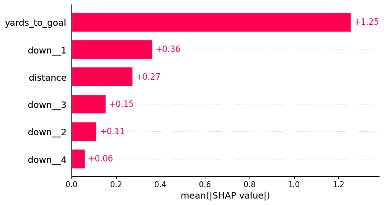
Explainability
We can use the Shapley values to identify the most important predictors like we did with the coefficients in the LASSO Regression. Also like the LASSO Regression, we see the same story as far as which variable is the most important, yards-to-goal.
import shap
explainer = shap.Explainer(xreg)
shap_values = explainer(X)
shap.plots.bar(shap_values)
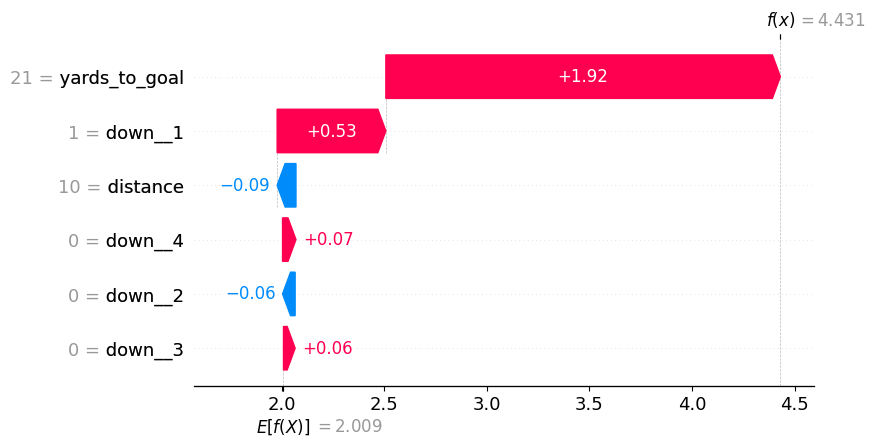
Some functionality that I love to use in the shap package is being able to look at an individual observation to see how the different predictors impact the final prediction. In the below image, we see that the model is predicting 4.4 points for the offensive team because they are running a play on 1st and 10 at the opponents 21-yardline.
from random import randint
random_play = randint(0, X.shape[0])
shap.plots.waterfall(shap_values[random_play])
Conclusion
In our evaluation of ML models for expected points prediction, we compared simple linear regression, lasso regression, and a boosted regression model. While all showed similar performance, lasso regression slightly outperformed the others. Its adeptness in handling multicollinearity proved advantageous in this dynamic context. Each model offers unique strengths, with simple linear regression's interpretability and the boosted model's ability to capture complex relationships. Overall, lasso regression stands as the top choice for its balanced performance and potential for practical application in NCAA football analytics.
While we are only able to explain 9% of the expected point variance with our selected variables and model, that's ok. We will seek to explain more of the variance with future models (e.g. offensive strength, defensive strength, homefield advantage, etc.). The purpose of this model will be to give a baseline that we can use to calculate the things like team strength and homefield advantage.